Tutorial
Welcome to the tutorial page! We are here to guide you through our web-based application step by step,
explaining the details as we go. All over the web pages you will also find shortcuts to the relevant
sections in the tutorial.
But for now, let’s get started from the top.
Readily accessible on our front page we give you the option to start a new ProteinLens session by clicking on the
Jump in button. This will get you straight to the
Input page.
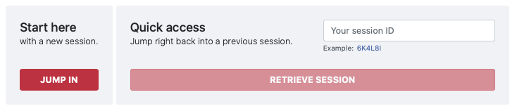
XXXXX_config.json file,
if you have already downloaded your results. Just enter this code and you will be directly forwarded to the Results page.
If you chose to start a new session, you will be directed to the input page.
In Pane 1 we ask you to provide the biological structure you want to explore.
Here you have two options:
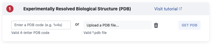
You can either get a structure directly from the Protein Data Bank (PDB) [06,07]
by entering its 4-letter code (left) or upload your own file (right).
If you decide to upload your own file, please make sure it is in the correct PDB format as
specified in
PDB’s Atomic Coordinate Entry Format Description (v3.3).
Once you specified a PDB code or uploaded your own file click on the Get PDB
button to get started.
Based on the contents of the PDB file you submitted, we give you some options in
Pane 2
before we construct the atomistic graph. The default settings select model 1 (in case of
multiple present) and all the chains identified in the input file. We also strip all
anisotropic temperature factors (ANISOU) entries, as they are not relevant for the graph
construction and
all water molecules, as they tend to disrupt the graph construction when they are too far
away from the rest of the structure.
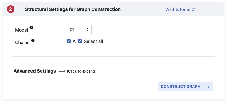
You can however modify your input through any or all of Model,
Chains or Advanded Settings
options, as explained below.
Model. If you have a structure which has several models, i.e. NMR structures (read more about NMR models on the PDB website, and about their biological meaning in [08]), you need to choose one model using this drop down menu. In cases where there is only one structure present, you can ignore this input parameter.
Chains. The next row of tick boxes allows you to choose the chains you want present
in your graph. Sometimes a PDB structure has several assemblies present and you might not
need all of them. Just tick the ones that are of interest to you. You can also select or
deselect all by using the Select all box.
Advanced Settings. For a first investigation of your biological structure, we recommend our default settings. However, if you would like to explore further and are familiar with PDB files, we have additional settings that allow you to decide what you would like to strip or keep in the input file.
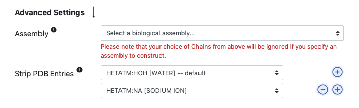
Many PDB files contain the minimal asymmetric unit necessary to construct the full macromolecule. For example, a given protein might be found experimentally to be a homodimer, but the authors might only solve (and report on the PDB) the structure of one chain, and include the coordinates of the atoms within it along with the symmetry transformations necessary to construct the full structure. We provide you with the option to choose the biological assembly you are interested in and automatically will model missing chains or strip unwanted chains. Please be aware that choosing this option will override your chain choice in Pane 2, as these parameters are mutually exclusive. You will find information on each assembly in the dropdown menu, such as which chains are included and the type of oligomer they form.
By default, all water molecules in the PDB file are stripped. However, if particular water
molecules are important, for example in the binding mode of a ligand, please provide your
own adjusted PDB file containing these water molecules, and, choose in the Advanced
Settings the option Don’t strip anything.
Using the blue plus and minus buttons on the left, you can add or delete more atom types to be stripped. You can also choose to strip all heteroatoms (HETATM), i.e. non-standard residue entries, at once.
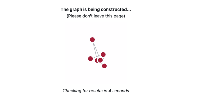
Once you are happy with all of your settings, click Construct Graph and we
will take care of the rest. Depending on the size of your structure, this might take up to
a minute, please be patient 😌
While your graph is constructed, you will see a waiting page which will automatically
refresh every 10 seconds.
- covalent bonds
- hydrogen bonds
- hydrophobic interactions
- salt bridges
- certain electrostatic interactions
- pi-pi stacking (in DNA)
A quick note here, we use REDUCE [12]
to add hydrogen atoms to PDB structures. By default we will strip all hydrogen atoms
present in the file and add them with REDUCE. If you should have a case in which you
want to leave your hydrogen atoms untouched, please contact us to discuss your options.
Once our algorithm constructs an atomistic graph of your structure we will give you some
feedback in Pane 1.
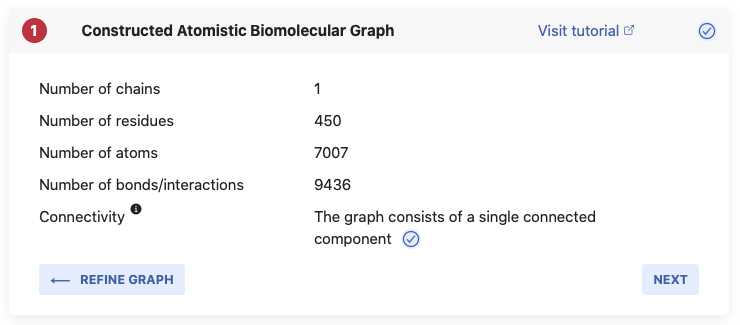
We will list the number of residues in the structure, the number of atoms (which equals the number of nodes in the graph), and the number of identified bonds/interactions, which is equal to the number of edges in the constructed graph. For our methods we need a connected graph, which means we cannot accept a graph in which any node or group of nodes is not connected to the graph over at least one bond. If you see a little blue tick, we have one connected graph and are good to continue.
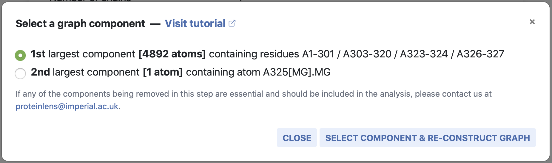
In cases where this is not true we give you the option of a quick fix:

By clicking on Quick Fix, a new window opens in which the disconnected graph
components are listed, ranked by their size in terms of number of atoms. This also
provides
information on the residues contained in each component and gives you the option to choose
the component that is relevant to you. The graph is then automatically re-constructed for
you.
In general you can always choose to go back to the input page to refine your settings. By
clicking Next the graph is accepted and we progress to choosing the source
residues in Pane 2.
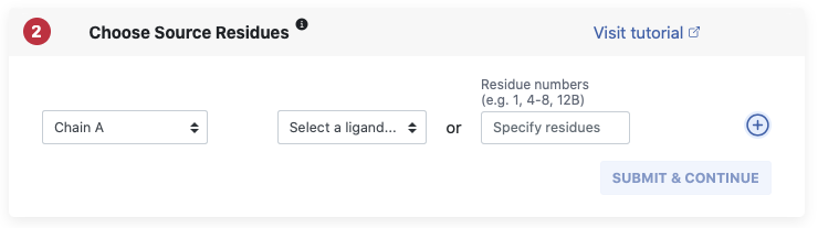
Our methods compute graph properties based on source residues. From a biological viewpoint the source is often the bound ligand in a binding side or a peptide which binds to a larger protein. You can specify your source residues on a certain chain by either choosing them from a dropdown menu, where all HETATOMs, i.e. non standard residues on this chain are listed. Alternatively, you can simple enter the residue numbers you want as your source on the chosen chain. With the blue plus and minus buttons on the left you can add residues on another chain in the same manner. Remark: You cannot choose more than 20% of your structure as source.
By clicking on Next you confirm your choice of source residues and pane
3
opens which is offering you the choice of methods:
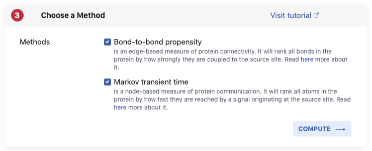
Using the tick boxes, you can choose from either Bond-to-bond propensity or Markov transient time or you can run both methods at once. Below the boxes you can see a short summary which provides a reminder about what our methods do. For more detail please make your way over to the Background page.
If your graph has more than 10,000 nodes (i.e. atoms) and you choose to compute Markov transient times, you will see a little remark to indicate that this method will take a little longer to compute on such a big graph, so please be patient and do not refresh the page.
Once you click Compute our methods will run in the background and you will be seeing
a waiting page which will refresh every 10 seconds. Once your computations are finished you will
automatically be forwarded to the results page.
And here they are, the results for your protein produced by our methods. But let’s look at
it piece by piece.
In a first step, we will give you a summary of your session in Pane 0 which
also gives you
the session ID to later recover these results.
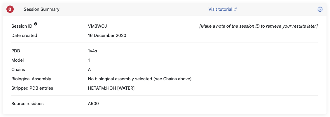
You will find information on the PDB file that was submitted, which model and chains you chose and which entries were stripped before graph construction. It will also give you a reminder of the source residues you chose. All this information can also be found in the config file that is in your download folder. We also state the session ID here, which will allow you to directly retrieve your results at a later point. You might want to write it down or you will also find in the above mentioned config file.
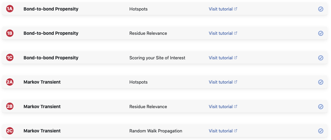
We present the results of Bond-to-bond propensity and Markov transients in five different
boxes. If the methods have been run and produced results, you will find a little blue
tick
on the left. If one of the methods has not been run, we provide a short cut button for you
to run them at this stage. Panes 1A and B belong to Bond-to-bond propensity
and
2A, B and C
to Markov transient. For both methods we provide an overview of the data patterns and the
found hotspots in the A Panes. The B Panes allow you to identify
significant residues at
different cut offs. But let’s look at this in more detail.
This view maps the quantile score of each residue in a color coded fashion onto your protein structure. The structure can be explored in an interactive manner and is fully linked to the results in the plot on the left. Hovering over a single residue on the right will yield a little window containing the data associated with this residue.
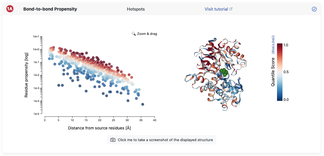
This view allows to investigate connectivity hotspots between the chosen source (shown in green) and the rest of the structure. More details on the mathematical significance of the quantile score can be found in the Background page.
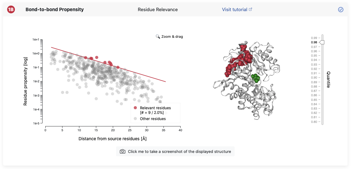
This view allows the investigation of residues that are significantly connected to the chosen source. Again, you find your structure on the right of the panel and it can be explored interactively by hovering over residues to get more information. The slider on the right can be adjusted for different significance thresholds and the respective residue will show up in dark red. The legend in the plot on the left additionally tells you how many residues are above your chosen threshold and what percentage they are of the whole structure. More details on the significance of the thresholds can be found in the Background page.
This view gives you the possibility to investigate your structure on the single residue level and identify the residues which are the most connected to your chosen source.
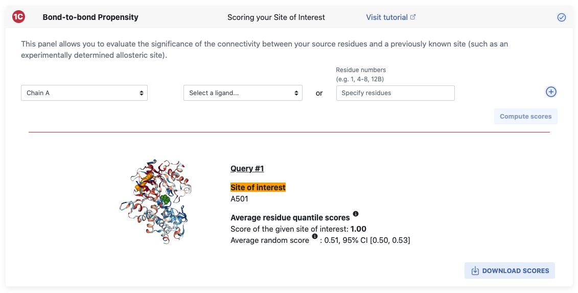
To aid you in further investigating your structure of interest, ProteinLens provides the opportunity to quantify the connectivity between the chosen source site and arbitrary sites of interest. After you’ve defined a potential site of interest (e.g. a known allosteric binding pocket), we use a random site generating algorithm to sample 1000 sites of the same size on your structure and a bootstrap to allow for statistical evaluation. Read more about this in the Background page.
The site of interest can be specified in the same fashion as the source site details were filled in.
Chain and ligands can be chosen from the dropdown menu or residue numbers can be specified directly.
Using the blue plus, you can add residues on a different chain as well.
Clicking on Compute scores will yield two 0-1 scores for your site of interest
(the residues in the site of interest will be shown in orange on your structure).
The two calculated scores are the average residue quantile score across your site of interest
and the average quantile score across 1000 randomly generated sites, which will be of the
same size as your input and can be anywhere on the structure. We also provide a 95% confidence
interval around the latter score to determine statistical significance. Comparing these two
scores allows you to infer the significance of your site of interest with respect to a site
picked at random. The score of your site is above the average random score? - Great! Your
site of interest is more connected to your source residues than a site picked at random.
By using the input fields again, you can investigate more sites which will be listed in the same fashion underneath.
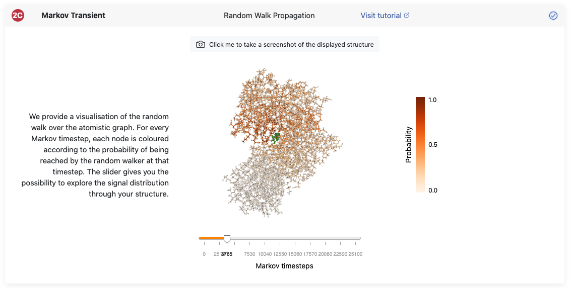
As detailed in the Background page, the computation of Markov transients is based on monitoring the progression of a random walker sourced on your residues of choice along the protein graph. This progression can be visualised by computing the probability of the random walker being on any of the nodes at a given time step. By using the slider on the bottom you can see interactively where the probability distributes sourced from your residues of choice. This view allows you to identify whether there are areas in your structure which have a more direct signal propagation towards them.
In each pane we provide the option to obtain a screenshot of the structure view by clicking the button on the bottom of each pane.
We also provide the option to download all your data when clicking on the
Download button.
The .zip file contains a range of raw files and raw data as well as result
plots which
are
all named according to the session:
sessionXXXXXX_README.md- gives an overview over all files and formats in this foldersessionXXXXXX_config.json- contains all the input options you chose in this sessionsessionXXXXXX_graph_atoms.csv- lists the atoms which were used as nodes in the constructed graphsessionXXXXXX_graph_bonds.csv- lists the bonds and interactions which were detected between all atoms and make up the edges in the constructed graphsessionXXXXXX_modified.pdb- the modified PDB file containing the chosen model, chains and only the atoms which have not been stripped offsessionXXXXXX_original.pdb- the original PDB file which has been uploaded by the user or downloaded from the PDBsessionXXXXXX_propensity_bonds.csv- results of the Bond-to-bond propensity calculations for all weak bonds present in the graphsessionXXXXXX_propensity_residues.csv- results of the Bond-to-bond propensity calculations for every residue of the biomoleculesessionXXXXXX_propensity_scores.csv- results of the scoring for all sites of interestsessionXXXXXX_transient_atoms.csv- results of the Markov transient calculations for atoms present in the graphsessionXXXXXX_transient_residues.csv- results of the Markov transient calculations for every residue of the biomolecule- Folder
sessionXXXXXX_propensity_plots- contains plots similar to the ones in panes 1A and 1B - Folder
sessionXXXXXX_transient_plots- contains plots similar to the ones in panes 2A and 2B